Note
This notebook can be downloaded here: 1D_interpolation.ipynb
1D interpolation
Scope
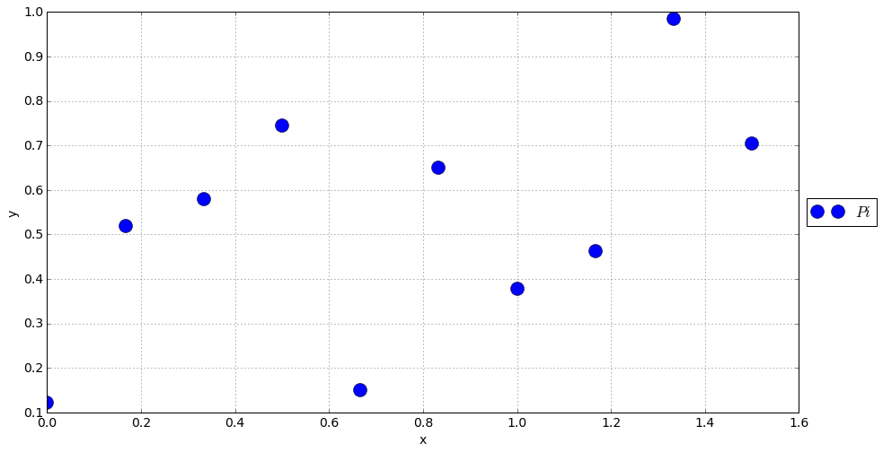
- Finite number \(N\) of data points are available: \(P_i = (x_i, y_i)\) , \(i \in \lbrace 0, \ldots, N \rbrace\)
- Interpolation is about filling the gaps by building back the function \(y(x)\)
https://en.wikipedia.org/wiki/Interpolation
# Setup
%matplotlib inline
import numpy as np
import matplotlib.pyplot as plt
import matplotlib
params = {'font.size'     : 14,
          'figure.figsize':(15.0, 8.0),
          'lines.linewidth': 2.,
          'lines.markersize': 15,}
matplotlib.rcParams.update(params)
Let’s do it with Python
N = 10
xmin, xmax = 0., 1.5
xi = np.linspace(xmin, xmax, N)
yi = np.random.rand(N)

plt.plot(xi,yi, 'o', label = "$Pi$")
plt.grid()
plt.xlabel("x")
plt.ylabel("y")
plt.legend(loc='center left', bbox_to_anchor=(1, 0.5))
plt.show()
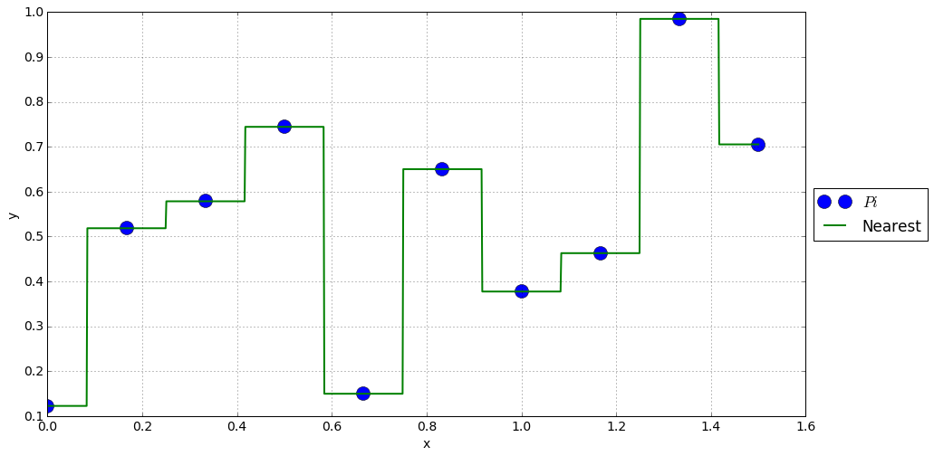
Nearest (aka. piecewise) interpolation
Function \(y(x)\) takes the value \(y_i\) of the nearest point \(P_i\) on the \(x\) direction.
from scipy import interpolate
x = np.linspace(xmin, xmax, 1000)
interp = interpolate.interp1d(xi, yi, kind = "nearest")
y_nearest = interp(x)

plt.plot(xi,yi, 'o', label = "$Pi$")
plt.plot(x, y_nearest, "-", label = "Nearest")
plt.grid()
plt.xlabel("x")
plt.ylabel("y")
plt.legend(loc='center left', bbox_to_anchor=(1, 0.5))
plt.show()
Pros
- \(y(x)\) only takes values of existing \(y_i\).
Cons
- Discontinuous
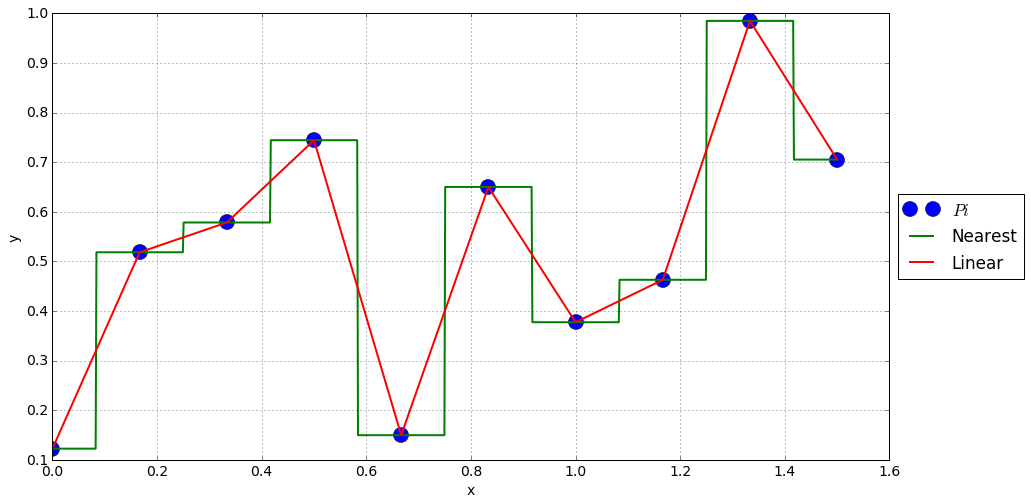
Linear interpolation
Function \(y(x)\) depends linearly on its closest neighbours.
from scipy import interpolate
x = np.linspace(xmin, xmax, 1000)
interp = interpolate.interp1d(xi, yi, kind = "linear")
y_linear = interp(x)

plt.plot(xi,yi, 'o', label = "$Pi$")
plt.plot(x, y_nearest, "-", label = "Nearest")
plt.plot(x, y_linear, "-", label = "Linear")
plt.grid()
plt.xlabel("x")
plt.ylabel("y")
plt.legend(loc='center left', bbox_to_anchor=(1, 0.5))
plt.show()
Pros
- \(y(x)\) stays in the limits of \(y_i\)
- Continuous
Cons
- Discontinuous first derivative.
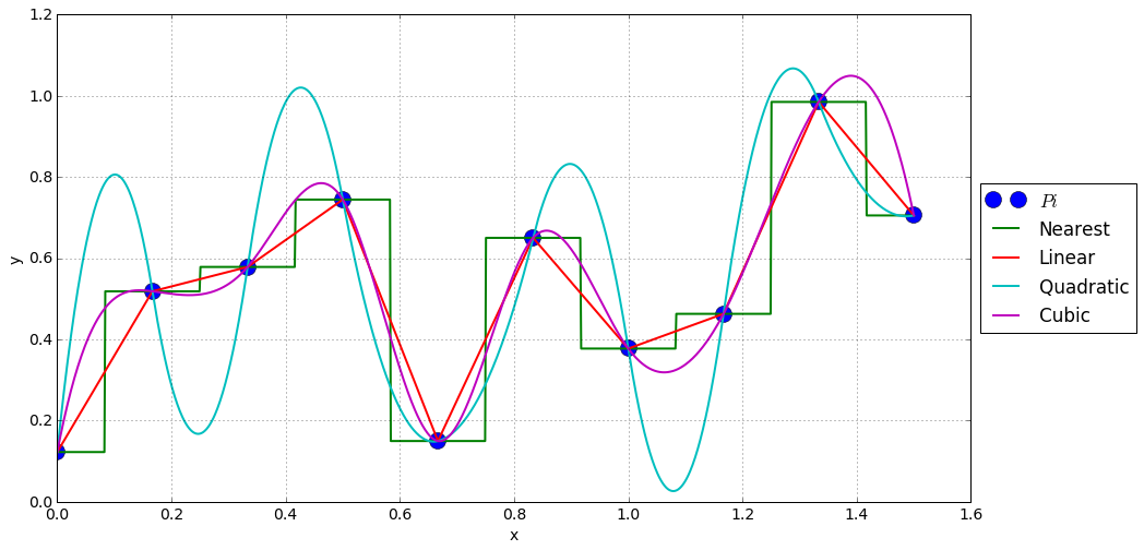
Spline interpolation
from scipy import interpolate
x = np.linspace(xmin, xmax, 1000)
interp2 = interpolate.interp1d(xi, yi, kind = "quadratic")
interp3 = interpolate.interp1d(xi, yi, kind = "cubic")
y_quad = interp2(x)
y_cubic = interp3(x)

plt.plot(xi,yi, 'o', label = "$Pi$")
plt.plot(x, y_nearest, "-", label = "Nearest")
plt.plot(x, y_linear,  "-", label = "Linear")
plt.plot(x, y_quad,    "-", label = "Quadratic")
plt.plot(x, y_cubic,   "-", label = "Cubic")
plt.grid()
plt.xlabel("x")
plt.ylabel("y")
plt.legend(loc='center left', bbox_to_anchor=(1, 0.5))
plt.show()
Pros
- Smoother
- Cubic generally more reliable that quadratic
Cons
- Less predictable values between points.