Tutorial 1: The simple pendulum¶

Introduction¶

This tutorial aims at modelling and solving the yet classical but not so simple problem of the pendulum. A representiation is given bellow (source: Wikipedia).

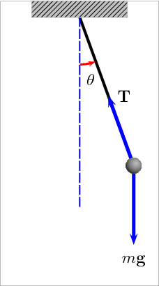
The simple pendulum

On a mechanical point of view, the point \(M\) with mass \(m\) is supposed to be concentrated at the lower end of the rigid arm. The length of the arm is noted \(l\). The frame \(R_0\) is assumed to be inertial. The angle between the arm and the vertical direction is noted \(\theta\). A simple modelling using dynamics leads to:

\[m\vec A(M/0) = \vec P + \vec T\]

Where:

\(\vec A(M/0)\) is the acceleration of the mass,
\(\vec P\) if the weight of the mass,
\(\vec T\) if the reaction force of the arm.

A projection of this equation along the direction perpendicular to the arm gives a more simple equation:

\[\ddot \theta = -\dfrac{g}{l} \sin \theta\]

This equation is a second order, non linear ODE. The closed form solution is only known when the equation is linearized by assuming that \(\theta\) is small enough to write that \(\sin \theta \approx \theta\). In this tutorial, we will solve this problem with a numerical approach that does not require such simplification.

# Setup
%matplotlib nbagg
import numpy as np
import pandas as pd
import matplotlib.pyplot as plt
from scipy.integrate import odeint

Numerical values¶

l = 1.   # m
g = 9.81 # m/s**2

Part 1: Reformulation of the problem¶

This problem can be reformulated to match the standard formulation \(\dot X = f(X, t)\):

\[\begin{split}X = \begin{bmatrix} \theta \\ \dot \theta \end{bmatrix} = \begin{bmatrix} x_0 \\ x_1 \end{bmatrix}\end{split}\]

Write the function \(f\) in Python:

def f(X, t):
    """
    The derivative function
    """
    # To be completed
    return

Part 2: Numerical solution at small angles¶

Solve the problem with Euler, RK4 and ODEint integrators and compare the results with the closed form solution. First assume that the pendulum is released with no speed (\(\dot \theta = 0 ^o/s\)) at \(\theta = 1 ^o\). The time discretization will be as follows:

duration: 10 s,
time step: 0.01 s.

def Euler(func, X0, t):
    """
    Euler integrator.
    """
    dt = t[1] - t[0]
    nt = len(t)
    X  = np.zeros([nt, len(X0)])
    X[0] = X0
    for i in range(nt-1):
        X[i+1] = X[i] + func(X[i], t[i]) * dt
    return X

def RK4(func, X0, t):
    """
    Runge and Kutta 4 integrator.
    """
    dt = t[1] - t[0]
    nt = len(t)
    X  = np.zeros([nt, len(X0)])
    X[0] = X0
    for i in range(nt-1):
        k1 = func(X[i], t[i])
        k2 = func(X[i] + dt/2. * k1, t[i] + dt/2.)
        k3 = func(X[i] + dt/2. * k2, t[i] + dt/2.)
        k4 = func(X[i] + dt    * k3, t[i] + dt)
        X[i+1] = X[i] + dt / 6. * (k1 + 2. * k2 + 2. * k3 + k4)
    return X

# ODEint is preloaded.

# Define the time vector t and the initial conditions X0

Part 3: Solution at large angles¶

Solve the problem with Euler, RK4 and ODEint integrators and compare the results with the closed form solution. First assume that the pendulum is released with no speed (\(\dot \theta = 0 ^o /s\)) at \(\theta \in [30 ^o, 90 ^o, 179 ^o]\).

Part 4: Solution at large angle with initial angular velocity¶

Solve the problem with Euler, RK4 and ODEint integrators and compare the results with the closed form solution. First assume that the pendulum is released with non zero initial angular velocity and \(\dot \theta = 179 ^o/s\).