Note

This notebook can be downloaded here: 00_Basics.ipynb

Basics

In this notebook, we introduce basic ways to read, show, explore and save images.

from PIL import Image
import numpy as np
import matplotlib.pyplot as plt
from matplotlib import cm
from scipy import ndimage
import os
%matplotlib nbagg

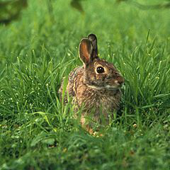
You can download the image used in this example here: rabbit.jpg. The following code will work if the image is located in the same directory as the notebook itself.

First, let’s check if the file rabbit.jpg is in the current directory.

files = os.listdir("./")
if "rabbit.jpg" in files:
    print("Ok, the file is in {0}".format(files))
else:
    print("The file is not in {0} , retry !".format(files))

Ok, the file is in ['rabbit.jpg', '.ipynb_checkpoints', '00_Basics.ipynb']

Now let’s read it using Python Image Library (aka PIL):

im = Image.open("rabbit.jpg")
im

Numerical images

There are mainly two kinds of numerical images:

• Vectorial images composed of basic geometric figures such as lines and polygons. They are very efficient to store schemes or curves. They are generally stored as .svg, .pfg or .eps files. In this tutorial, we will not work on such images.
• Raster images, also called bitmaps in which data is structures as matrix of pixels. Each pixel can contain from 1 to 4 values called channels. Images can then be sub classed by their number of channels:
  • A single channel image is called grayscale,
  • Most color images use 3 channels, one for red (R), one for green (G) and one for blue (B). They are called RGB images.
  • Some image formats use a fourth channel called alpha corresponding to the transparency level of a given pixel.

In the current image, the channel structure can be obtained as follows:

im.getbands()

('R', 'G', 'B')

From image to numpy

Now, the channel data can be extracted as follows:

R, G, B = im.split()
R = np.array(R)
G = np.array(G)
B = np.array(B)
R

array([[ 78,  85,  96, ...,  79,  70,  64],
       [ 72,  76,  84, ...,  99,  93,  89],
       [ 69,  71,  75, ..., 108, 101,  95],
       ...,
       [120, 115, 101, ...,  73,  64,  38],
       [130, 109,  80, ...,  73,  58,  31],
       [113,  84,  60, ...,  72,  68,  53]], dtype=uint8)

fig = plt.figure()
ax1 = fig.add_subplot(1, 3, 1)
plt.title("R")
plt.imshow(R, cmap = cm.gray)
ax1.axis("off")
ax1 = fig.add_subplot(1, 3, 2)
plt.title("G")
plt.imshow(G, cmap = cm.gray)
ax1.axis("off")
ax1 = fig.add_subplot(1, 3, 3)
plt.title("B")
plt.imshow(B, cmap = cm.gray)
ax1.axis("off")
plt.show()

<IPython.core.display.Javascript object>

From numpy to image

Let’s now see how we can create an image from numpy.

r2 = np.arange(256).astype(np.uint8)
g2 = np.arange(256).astype(np.uint8)
R2, G2 = np.meshgrid(r2, g2)
B2 = np.zeros_like(R2).astype(np.uint8)

im2 = Image.fromarray(np.dstack([R2, G2, B2]))
im2

Let’s apply that to the rabbit image. For example, we can switch channels:

im3 = Image.fromarray(np.dstack([G, R, B]))
im3